This tutorial holds the example analysis to estimate gradients for simulation data (Simulation1 in the paper).
1. Simulate data
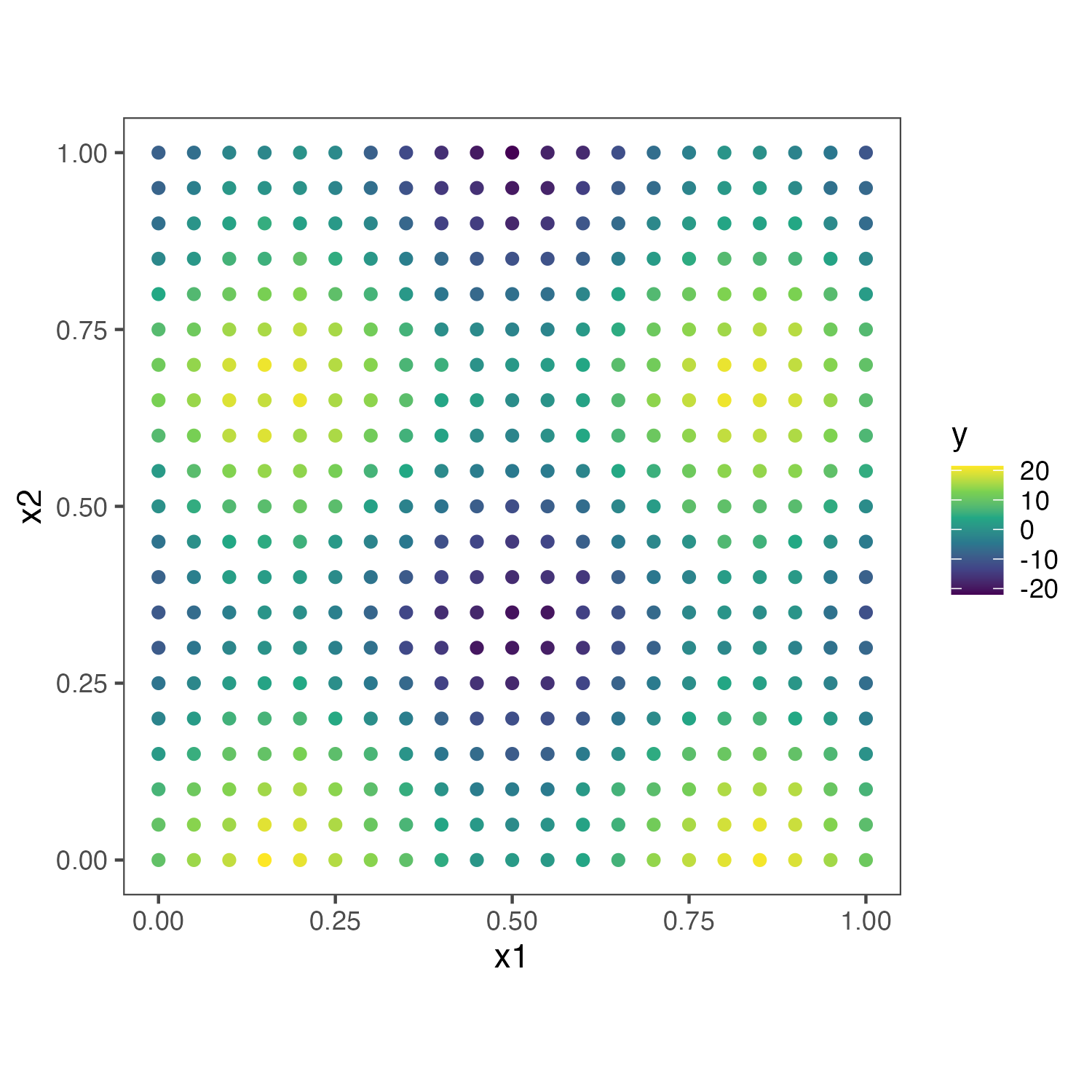
For simulation1, we simulate \(y \sim 10 N(sin(3\pi x_1)+cos(3\pi x_2),1)\) .
library(dplyr)
library(data.table)
library(ggplot2)
library(cowplot)
library(ggsci)
library(egg)
library(paletteer)

rmvn <- function(n, mu=0, V = matrix(1)){
    p <- length(mu)
    if(any(is.na(match(dim(V),p))))
    stop("Dimension problem!")
    D <- chol(V)
    t(matrix(rnorm(n*p), ncol=p)%*%D + rep(mu,rep(n,p)))
}

##Make some data
set.seed(1)
N <- 100
tau <- 1
# synthetic location
#coords <- matrix(runif(2*N),nr=N,nc=2)

coords_x = seq(0,1,0.05)
coords_y = seq(0,1,0.05)
coords = expand.grid(coords_x,coords_y) %>% as.matrix()

# synthetic pattern
y <- rnorm(nrow(coords),10*(sin(3*pi*coords[,1])+cos(3*pi*coords[,2])),tau)
2. Fit Nearest-Neighbor Gaussian Process (NNGP) model
library(StarTrail)
thread = 1 # number of CPUs to use
m.r = fit_NNGP(coords,y,neighbor = 10,threads = thread) # here we use 10 neighbors
3. Calculate gradients
# minimal separation of training data coordiantes
min_sep = 0.05
# gradient at the orignial resolution
gradient_all = finite_difference(coords, # coordinate of the point you wanna calculate the gradient on e1 and e2
min_sep*0.8, # h: minimal separation
m.r, # fitted NNGP model
threads=thread, # cpu to use
prefix = 'ori', # file prefix of saved file
path=path,# path to save files
save_file = FALSE,
verbose = FALSE # print progress
)
gradient_all = cbind(coords,y,gradient_all)
colnames(gradient_all) = c('s1','s2','y','pred','g1','g2','g1_min','g1_max','g2_min','g2_max')
# s1: first item of coord (x1), s2: first item of coord (x2)
# y: truth, pred: predicted y
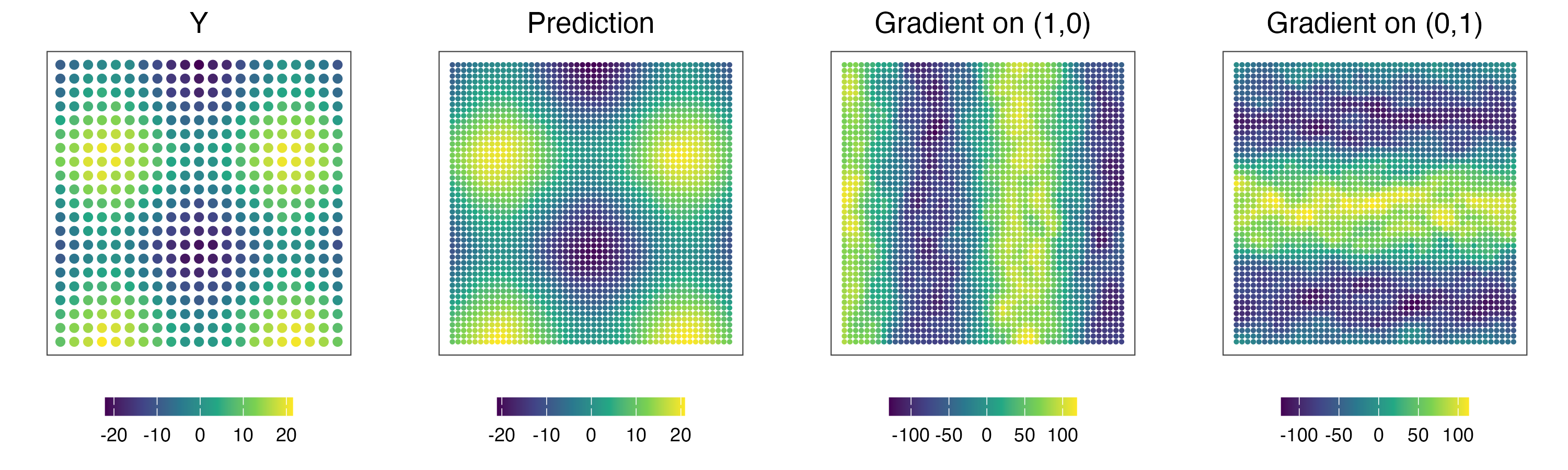
# g1: gradient on (1,0), g2: gradient on (0,1)
# g1_min, g1_max, g2_min, g2_max: posterior min and max for g1 and g2
Here are the estimated gradients.
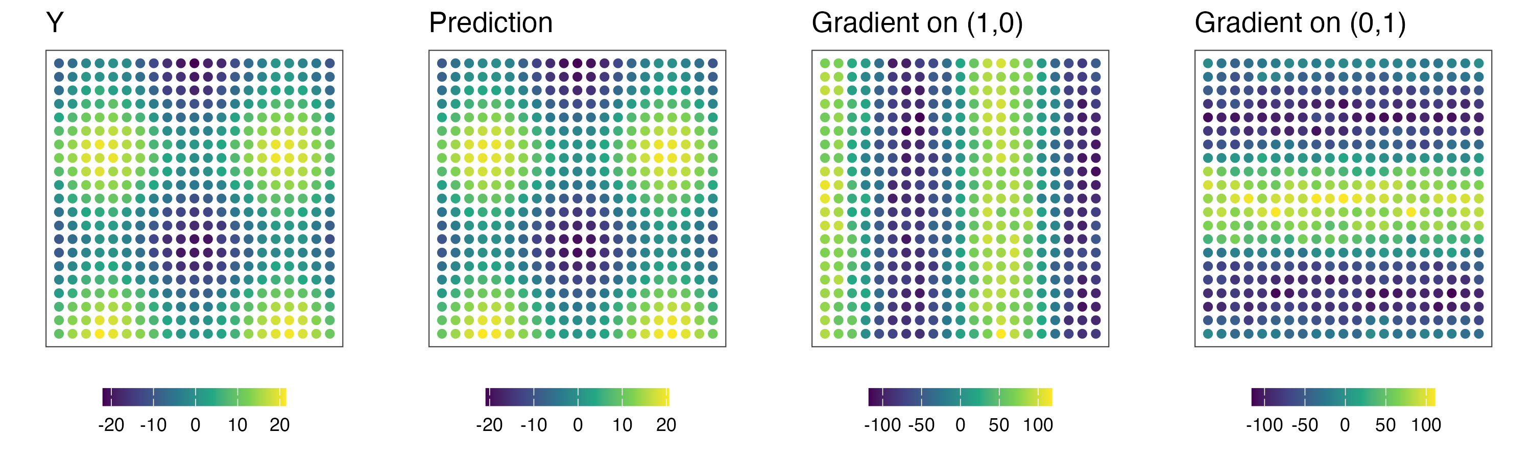
4. Increase resolution
# coordinates at the increased resolutionå
coord_mesh_x = seq(min(coords[,1]),max(coords[,1]),length.out=50)
coord_mesh_y = seq(min(coords[,2]),max(coords[,2]),length.out=50)
coord_mesh = expand.grid(coord_mesh_x,coord_mesh_y) %>% as.matrix()

gradient_mesh = finite_difference(coord_mesh,min_sep*0.8,m.r,threads=thread,prefix = 'mesh',path=path,verbose = FALSE)
gradient_mesh = cbind(coord_mesh,gradient_mesh)
colnames(gradient_mesh) = c('s1','s2','pred','g1','g2','g1_min','g1_max','g2_min','g2_max')